Type of reactions simulated in module MET&OR

• Definition of a reaction : reaction affects one or more “reactive” variables. The reaction rate R regulates the flux of material exchanged between these variables or the flux of material which is created or which disappears due to this reaction.

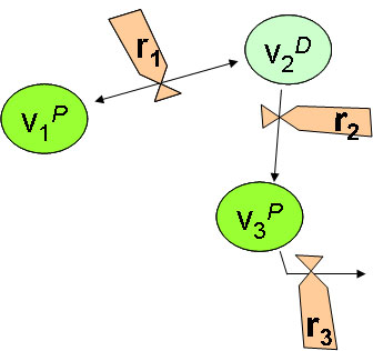
• 5 reaction types :

  • 1 REAC_1 : first-order reaction affecting one single variable (First order reaction (REAC_1))
  • 2 Generic : reaction between several variables, with limiting functions (Multiple and limited reaction (Generic))
  • 3 reversible : reversible reaction between two variables (Reversible reaction (REVERS))
  • 4 PART_EQ : sorption reaction at equilibrium between several variables (Partitioning reaction at equilibrium (PART_EQ))
  • 5 volatilization : reaction for volatil substance, dissolved in water column (2 layers model of Liss and Slater, 1974) (Volatilization (VOLATIL))

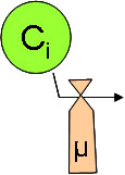
First order reaction (REAC_1)

The “REAC_1” reaction is a simple reaction, like first-order degradation, affecting one single variable with a constant kinetic (but still varying with temperature) and a stoichiometric coefficient.

\(\frac{\partial C_i}{\partial t}= \alpha_i R_1\) \(R_1=\mu_1 F_{Temp} C_i\) \(C_i\) : reactive variable concentration \(\alpha_i\) : stochiometric constant \(\alpha_i <0\) if Ris a sink for variable i \(\mu_1\) : reaction kinetic (1/T) at reference temperature \(F_{Temp}\) : Arrhenius function (Kinetic Modulation with Temperature (Arrhenius function) ) modulate reaction cinetic according to temperature

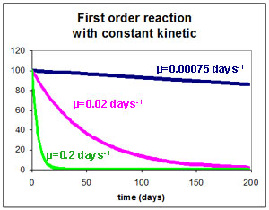
Exemple : radioactive decroissance \(\frac{\partial C_i}{\partial t}= -\mu C_i\) with \(\mu\) : reaction kinetic Reaction kinetic \(\mu\) is related to T90 by \(C_{t=T_{90}}=0.1 C_{t=0} \Rightarrow \mu=\frac{2.3}{T_{90}}\) and to T50 by \(C_{t=T_{50}}=0.5 C_{t=0} \Rightarrow \mu=\frac{0.69}{T_{50}}\)

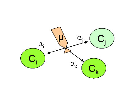
Multiple and limited reaction (Generic)

The so-called “generic” reaction includes a number of reactions describing the interaction between several variables. It includes a maximum kinetic µ (at the reference temperature) which may be limited by various parameters (Kinetic Modulation with Temperature (Arrhenius function) or limiting functions of different types : Kinetic Limitation with a Monod function or an inhibiting function or with light radiation ). The exchange term R may depend upon the concentration of one or more different variables.

with 3 reactive variables : \(\frac{\partial C_i}{\partial t}= \alpha_i R_2\) \(\frac{\partial C_j}{\partial t}= \alpha_j R_2\) \(\frac{\partial C_k}{\partial t}= \alpha_k R_2\) \(R_2=\mu_2 F_{Temp} \sqcap{F_L} C_i^n C_j^m C_k^p\) \(C_{i,j,k}\) : reactives variables concentrations \(n,m,p\) : exponent of each reactive variable \(\alpha_{i,j,k}\) : stochiometric constants \(\alpha_{i,j,k} <0\) if Ris a sink for variable i, j or k \(\mu_{2}\) : reaction kinetic (1/T) at reference temperature \(F_{Temp}\) : Arrhenius function (Kinetic Modulation with Temperature (Arrhenius function) ) modulate reaction cinetic according to temperature \(F_{L}\) : Kinetic Limiting functions [0-1] Kinetic Limitation with a Monod function or an inhibiting function or with light radiation

Exemple : nitrification, bacterial growth, bacterial mortality...

Reversible reaction (REVERS)

This type of reaction deals with a reversible exchange between two variables managed by a rate constant and equilibrium concentration.

\(A\stackrel{\mu_1\rightarrow}{\leftarrow\mu_2} B\)

\(\frac{\partial A}{\partial t}=-\mu_1 A + \mu_2 B\)

\(\frac{\partial B}{\partial t}=\mu_1 A - \mu_2 B\)

These reactions may be treated as “generic” reactions, with μ1 μ2 as kinetics; but in some cases, the rate constant (sum of the two kinetic) and equilibrium concentration of a reactive variable is is better known. In the simple case of two active variables and an first order evolution , we can write:

\(\frac{\partial A}{\partial t}=-K (A-A_{eq})= K (B-B_{eq})=-K(A-\frac{B_{eq}}{r})\)

\(\frac{\partial B}{\partial t}=K (A-A_{eq})= -K (B-B_{eq})=K(A-\frac{B_{eq}}{r})\)

avec

• \(K=\mu_1 + \mu_2\) : rate constant(1/T)
• \(A_{eq}=\frac{A+B}{1+r}\) : concentration at equilibrium of variable A (M/V)
• \(B_{eq}=r\frac{A+B}{1+r}\) : concentration at equilibrium of variable B (M/V)
• \(r=\frac{\mu_1}{\mu_2}=\frac{B_{eq}}{A_{eq}}\) : concentration at equilibrium of variable B (M/V)

The rate of these reactions may vary according to the temperature in the same manner as the reactions of type 1 and 2.

Reaction 3 can be written in a more general way :

\(\frac{\partial C_i}{\partial t}=\alpha_i R_3\)

\(\frac{\partial C_j}{\partial t}=\alpha_j R_3\)

\(R_3=\mu_3 F_{Temp} (C_i - C_i^{equ})\)

avec

• \(C_i\) : first reactive variable, (called “active”) one whose equilibrium constant is known
• \(C_j\) : second reactive variable
• \(C_i^{equ}\) : equilibrium concentration of the first variable reactive Ci
• \(\alpha_i=-1\) : sign of reaction relative to the variable Ci
• \(\alpha_j\) : stochiometric coefficient relative to the variable Cj
• \(\mu_3\) : rate constant
• \(F_{Temp}\) : Arrhenius function (Kinetic Modulation with Temperature (Arrhenius function) )

Partitioning reaction at equilibrium (PART_EQ)

These reactions deal with the equilibrium partitioning between several variables that undergo rapid and reversible reaction for which we consider that the equilibrium is reached. These reactions are most often of the adsorption / desorption reactions.

There are two possibilities :

• Linear Equilibrium (Linear Partitioning reaction at equilibrium :)
• Non Linear Equilibrium (not supported in MET&OR)

In all cases, the equilibrium is achieved and the concentration of each variable is calculated from the linear partitioning coefficients for linear domains.

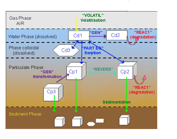
Volatilization (VOLATIL)

This reaction can take into account the exchange to the air / water interface of some so-called “volatil” variables. This process is a major process in the environment for a number of organic compounds. The most classical and commonly used theory to express this process is that proposed in the two-layer model (Liss and Slater, 1974) based on the Whitman two-film resistance model (1923). A number of parameters are required and a choice of formulas is proposed to assess exchanges in liquid and gaseous phases.

This reaction is written in the generalized form :

\(\frac{\partial C_w(i)}{\partial t}=\frac{F}{z}=\frac{K_{ol}(i)}{z}[C_w(i)-\frac{C_a(i)}{H'_T(i)}]\)

avec :

• \(C_w(i)\) = concentration in water (M/V)
• \(C_a(i)\) = concentration in air (M/V)
• \(z\) = depth of the layer
• \(K_{ol}\) = overall mass transfer coefficient (L/T)
• \(H'_T(i)\) = dimensionless Henry law constant

The overall mass transfer coefficient is estimated by :

\(K_{ol}(i)=\frac{k_l(i) k_g(i) H'_T(i)}{H'_T(i) k_g(i) + k_l(i)}\)

avec :

• \(k_l(i)\) = liquid-film transfer coefficient (L/T)
• \(k_g(i)\) = gas-film transfer coefficient (L/T);
• \(H'_T(i)\) = dimensionless Henry law constant depending on température T (T in °K)

Transfer coefficients \(k_l\) and \(k_g\) are evaluated from the mass transfer coefficients measured for reference compounds :

\(k_{l}(i)=k_l(R_l)\frac{Y_l(i)}{Y_l(R_l)}^{n_l}\)

\(k_{g}(i)=k_g(R_g)\frac{Y_g(i)}{Y_g(R_g)}^{n_g}\)

avec :

• \(R_l\) = reference compound used for resistance in liquid phase
• \(R_g\) = reference compound used for resistance in gaz phase
• \(Y_l(i)\) or \(Y_l(R_l)\) = parameter to correct the mass transfer in the liquid phase (molar mass or diffusivity or Schmidt number)
• \(Y_g(i)\) or \(Y_g(R_g)\) = parameter to correct the mass transfer in the gaz phase (molar mass or diffusivity)
• \(n_l\) and \(n_g\) = exponents of proportionality ratio for the resistance in the liquid phase and in the gaz phase

Reference compounds \(R_l\) and \(R_g\) choose to determine mass transfer coefficients in the liquid and gas phases depend on the data available for each contaminant.

• For the gas phase, the most used compound is water: \(X_g=H_2O\)
• For the liquid phase, the most used compound is carbonic gaz: \(X_l=CO_2\)
• Choice of formulations and parameters for transfert coefficients evaluation are presented in Volatilization : Transfert coefficients

Concentration in air of the compounds i is supposed to be constant and uniform. Its value is given in input file variable.dat

Henry law constant is given either in dimensional form (H), either in its dimensionless form. In the first case, the dimensionless value H’ will be automatically calculated by dividing H by the universal gas constant R and the temperature T (in ° K). Henry’s constant is then corrected for temperature and salinity :

\(H'_T=H'_{20degC} 10^{-B(\frac{1}{T}-\frac{1}{293})}\) (Staudinger & Roberts (2001)

\(H_Sal=H_{Sal=0} 10^{\alpha S}\) (Schwarzenbach et al, 1993, Totten et al, 2001, Xie et al, 2005)

avec :

• \(H'_{20degC}\) = dimensionless Henry law constant at 20 degres Celcius
• \(B\) = slope (deg Kelvin) expressing the variation of H’ as a function of temperature (Staudinger & Roberts (2001)
• \(alpha\) = Setschenov constant or salting out constant

• Linear Partitioning reaction at equilibrium :
• Volatilization : Transfert coefficients