Formulations of sediment module SEDI_MARS3D
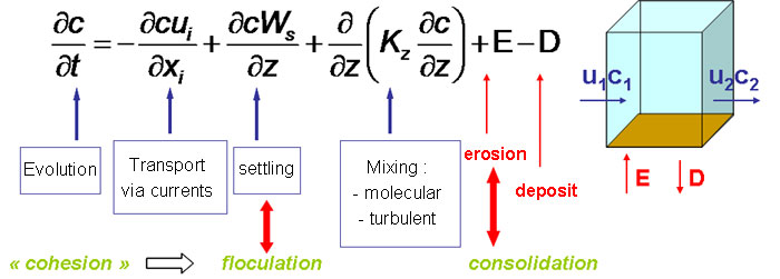
Erosion Process \(=f_1(\tau_s,\tau_e, composition\ density\ of\ sediment\ surface)\)
Deposit Process \(=W_s . f_2(\tau_s,\tau_d). C_{bottom\ extrapolated}\)
Setlling Process \(W_s=f_3(C,turbulence,salinity)\)
Erosion Process \(\tau_e=f_4(consolidation)\)
- Bioturbation within sediment (not operational)
There are 2 options (2 strategies) : key_sedim_mudsand or key_sedim_mixsed. but, this last option key_sedim_mixsed is highly recommended and the only one presented in this documentation. The new module MUSTANG (which will replace SEDI-MARS) only use the option key_sedim_mixsed (Module Sediment MUSTANG).
- The different computation steps for sediment module are :
- computing bottom shear stress \(=\tau_s\) f(U,waves, roughness)(Erosion Process)
- computing settling rate in water column (Setlling Process) and (Settling velocities : Modelling strategy)
- computing settling trends (Setlling Process)
- extrapolation of sand concentration near bottom (Extrapolation of sand variable near bottom (Rouse profile))
- sediment consolidation and diffusion into sediment layers (Consolidation of sediment and Diffusion within sediment and at interface)
- computing total mass eroded and suspending (Erosion Process)
- after particules transport in water column, computing of effective deposit, updating sediment layers (Deposit Process)
Erosion Process
Erosion flux E :
\(E=E_0*\alpha*[\frac{\tau-\tau_{ce}}{\tau_{ce}}]^n\)
- \(E_0\) and n depend on the mud fraction in sediment
- \(fr_{mud} < frv1\) : sandy sediment (frv1=0.3 typically = frmudcr1 calculated from coef_frmudcr1 in parasedim.txt)
- \(fr_{mud} > frv2\) : muddy sediment (frv2=0.7 typically = frmudcr2 given in parasedim.txt)
the critical erosion shear stress of erosion \(\tau_{ce}\) depends on the content of sand / mud and on sediment consolidation. It may be modulated by heterometry (hide / show)
- \(\alpha\) is a correction factor
- \(\alpha=1.+corfluer1*\max(0,corfluer2-Csed_{total-surf})\) (corfluer1 et corfluer2 given in parasedim.txt)
- For muddy sediment :
- \(E_0=E0_{mud}\) (given in parasedim.txt)
- \(\tau_{ce}=x1_{toce}* C_{mud}^{neros_{mud}}\) (parameters given in parasedim.txt)
- For sandy sediment :
\(E_0=E0_{sand}\)
- \(E0_{sand}\) given in parasedim.txt or estimated by formulations depending on the option chosen
E0_sand_option = 0 ==> E0_sand= E0_sand_para read in this namelist parasedim.txt
E0_sand_option = 1 ==> E0_sand evaluated with Van Rijn (1984) formulation
E0_sand_option = 2 ==> E0_sand evaluated with erodimetry formulation
\(E0_{sand}=\min(0.27,1000*d50-0.01)*(\tau-\tau_{ce})^{n_{eros-sand}}\)
\(\tau_{ce}=\) estimated from sand characteristics
For sand/mud mixing : Erosion flux depends on proportions of the mixture
Note
Several options are available but all are questionable and should be tested and used carefully
- The option choice is given by ero_option in parasedim.txt
- ero_option = 0 : pure mud behavior (for all particles and whatever the mixture)
- ero_option = 1 : linear interpolation between sand and mud behavior, depend on proportions of the mixture
- ero_option = 2 : formulation derived from that of J. Vareilles (2013)
- ero_option = 3 : formulations proposed by B. Mengual (2015) with exponential coefficients depend on proportions of the mixture
Erosion flux is applied in proportion to the mass of the considered fraction of sediment
- A lateral erosion process of a wet or dry cell was introduced into the model.
- Parameters coef_erolat, l_erolat_wet_cell and coef_tenfon_lat are used for this option., given in parasedim.txt
dry cell :\(Ero_{lat}=(\alpha_{lat} * U_{neighb}^2-\tau_{ce})*H_{neighb}\)wet cell (if l_erolat_wet_cell = .TRUE.)\(Ero_{lat}=(\beta_{lat} * \alpha_{lat} * U_{neighb}^2-\tau_{ce})*\delta_H\)with \(\alpha_{lat}\) =coef_tenfon_latwith \(\beta_{lat}\) =coef_erolatwith \(U_{neighb}\) =water current in the neigboring cellwith \(H_{neighb}\) =depth in the neighboring cellwith \(\delta_H\) =depth difference between eroded cell and the neighboring
Deposit Process
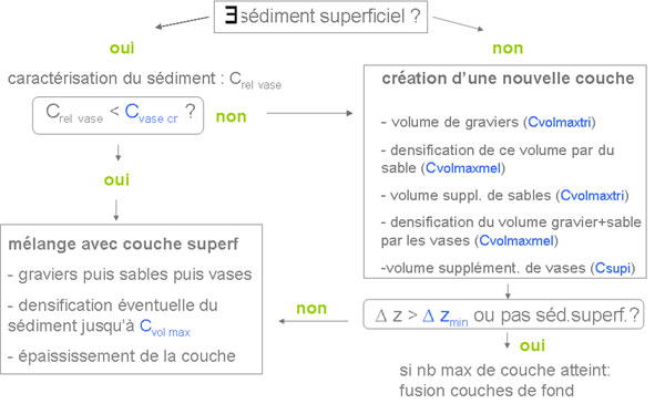
- first deposit of gravels, then sands, then muds
- deposit is caracterised by the mass fraction of each variable ( \(f_{rdep}(iv)\) )
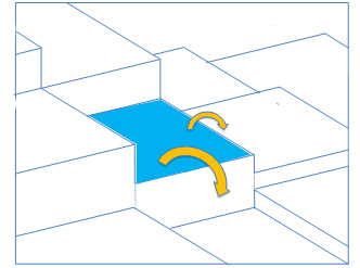
- A sliding process of the fluid mud was introduced into the model; mud slides if the slope is steep and deposits towards lower neighboring cells according to the slope
Setlling Process
Settling process depend on settling velocity, which varies according to the particulate material.
a modelling strategy is proposed with a choice of some formulations for defining the settling velocity W_s for MUD variables. (Settling velocities : Modelling strategy).
SAND variable have settling velocities W_s wich depend on particle diameter.
None constitutive SORBED variables have the same settling velocity as the associated constitutives particulate variable.
For the none constitutive variables which are not sorbed on constitutive particulate variable (type NoCP), settling velocity is evaluated in the same manner as MUD variables.
- Settling processes are treated implicitly in water transport equations.
- First, deposition flux trends are evaluated for each variable before advection computations :\(Fl_{w2s}^a= W_s . f_2(\tau_s,\tau_d)\) (m/s)Then after advection resolution, effective deposit is computed with new concentrations in water\(Fl_{w2s}^b= Fl_{w2s}^a*C_{bottom}\) (Masse/m2/s)and sediment layers are updated
For variables which have high settling velocity, vertical transport is computed using several sub time step in order to avoid instabilities.
Extrapolation of sand variable near bottom (Rouse profile)
Treatment of sand as 2D variable in water column (key_sandbottomcell)
Diffusion within sediment and at interface
Diffusion into the sediment is computed resolving following equations 1 (after Consolidation of sediment processes or not)
\(\frac{\partial (dzs_k*\varphi_k*Cs_k)}{\partial t}=+F_k-F_{k-1}\) (Equation 1A)\(F_k=\phi i_k^{t+dt}*Ds_k*\frac{Cs_{k+1}^{t+dt}-Cs_{k}^{t+dt}}{dzsi_k}-Wsi_k*(c_{ex}Cs_{k+1}^{t+dt}+f_{ex}Cs_{k}^{t+dt})\) (Equation 1B)- with :
- \(Cs_k^{t+dt}\) : dissolved substance concentration into layer k and at time t+dt (Mass/m^3[pw] [pw:pore water])
- \(F_k\) : Flux at interface between layer k and layer k+1 (Mass/T/m^2[sed])
- \(dzs_k\) : thickness of layer k (m[sed])
- \(dzsi_k\) : intermediate thickness between Cs_k and Cs_{k+1} (m[sed])
- \(\varphi_k^{t}\) : porosity into the layer k at time t (m^3[pw]/m^3[sed])
- \(\phi i_k^{t}\) : intermediate porosity at the interface between the layer k and the layer k+1 at time t (m^3[pw]/m^3[sed])
- \(Ds_k\) : Effective dispersion coefficient (m^2[sed]/T), corrected by tortuosity \(\theta\) (see Eq 1C)
- \(Wsi_k\) : transfert rate of pore water at the interface between the layer k and the layer k+1 [m^3[pw]/m^2[sed]/T)
- \(f_{ex},c_{ex}\) : factors upstream decentering for advection (\(f_{ex}=1\) : completely upstream evaluation)
- \(Ds_k=\frac{D_0}{\theta^2}\) and \(\theta^2=1-\ln(\varphi^2)=1-2*ln(\varphi)\) (Boudreau,1997)
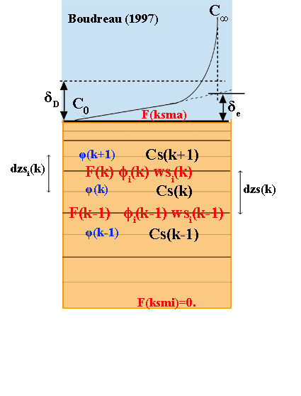
At bottom , F(k-1)=0.
- At sediment surface (water-sediment interface) (k=ksmax) :
\(F_k=\beta (C_{wat}^{t+dt}-Cs_k^{t+dt}) - Wsi_k*Cs_k^{t+dt}\)
- Three expressions are proposed here (dependent of choice_flx_diffsed given in parasedim.txt)
- choice_flx_diffsed given =1 : Fick law with diffusive sublayer supposed to be = half the thickness of the bottom layer
- ==>> \(\beta=2.*\frac{Ds_k}{dzsi_{ksmax}+dz(1)}\)
- choice_flx_diffsed given =2 : Fick law with diffusive sublayer supposed to be = distance epdifi (given in parasedim.txt)
- ==>> \(\beta=\frac{Ds_k}{0.5*dzsi_{ksmax}+epdifi}\)
- choice_flx_diffsed given =3 : formulation proposed by Boudreau (1997)
- ==>> \(\beta=\frac{Ds_k}{\delta_e}\)
- \(\delta_e\) : thickness of an effective diffusive sublayer that has a completely linear gradient and has the same flux as the real diffusive sublayer of thickness \(\delta_e\) (see fig)
- \(\beta=0.0889 U_* Sc^{-0.704}\) : formulation of Shaw and Hanratty (1977) in Boudreau (1997) (U_* is the shear velocity and Sc is the Schmidt number)
Bioturbation within sediment
Bioturbation is the result of all activities of the meio and macro-fauna living in the water-sediment interface or in the upper layers of the sediment.
- Bioturbation processes include :
- “surface biodiffusion”
- resulting of benthic organisms living in the first centimeters of the sediment. | Their movement causes the mechanical homogenization of the substrate and randomly in three dimensions;
- “bioirrigation”
- generated by agencies that construct galleries or burrows in the sediment.
These biodiffuseurs gallery provide irrigation sediment creating water currents to respiratory and food purposes.
- “bioadvection”
- induced by organisms that ingest sediment particles in depth (anoxic zone) and discharge their fecal pellets on the sediment surface.
This transport facing up induces a direct link between two non-adjacent geochemical and different strata. The bioadvection may also be downwardly directed
- But in a first step, bioturbation is considered here only as an apparent biodiffusion mixing coefficient Db.
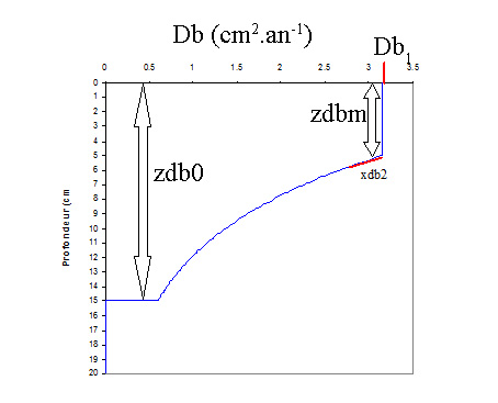
- The coefficient Db at each point and in each sediment layer is evaluated based on an average profile
with a maximum bioturbation intensity (Db1 in m^2.s^-1) near the interface to a specified depth (zdbm, m), then a decrease in depth according to a slope coefficient (xdb2 without unit) to a maximum depth of bioturbation (zdb0 in m), beyond which the bioturbation is considered null (Figure)
Note
These processes are available in SEDIMARS but not operational. They mus be tested and developped by researchers.
For dissolved substances, bioturbation processes are resolved simultaneously with the diffusion process in the sediment (diffusion routine)
- For particulate substances,
- either bioturbation processes are not involved
- or (to be checked) resolved simultaneously with the consolidation process, but explicitly in time with fractionnary time step; and if consolidation is not taking account, bioturbation for particulate variables are resolved alone in the consolidation routine.
- Parameters for bioturbation are given in parasedim.txt (namelist for sediment : parasedim.txt)
- l_bioturb : boolean set to .true. si taking into account bioturbation diffusion in sedimentxbioturbmax : max diffusion coefficient by bioturbation Db (in surface)xbioturbk : coef (slope) for bioturbation coefficient between max Db at sediment surface and 0 at bottomdbiotu0 : max depth beneath the sediment surface below which there is no bioturbationdbiotum : sediment thickness wherein the diffusion-bioturbation coefficient Db is constant (max)frmud_db_min : mud fraction limit (min) below which there is no Bioturbationfrmud_db_max : mud fraction limit (max) above which the bioturbation coefficient Db is maximum (muddy sediment)
Consolidation of sediment
The mixed-sediment consolidation model, detailed in Grasso et al. (submitted), is based on Toorman’s (1996) unifying theory for sedimentation and consolidation of several classes of sediment.
Following Merckelbach’s derivation of Gibson equation, and using as state variable the mass concentration of each sediment class Ci, the mass conservation equation during consolidation can be written as:
\(\frac{\partial C_i}{\partial t}=+\frac{\partial}{\partial z} [\frac{k}{\rho_w}C_i \triangle (load)]\) (Equation 2)
with
\(\triangle (load)=C \frac{\rho_s - \rho_w}{\rho_s} + \frac{1}{g} \frac{\partial \sigma'}{\partial z}\)
- where :
- C is the sediment total mass concentration, assuming the same grain density \(\rho_s\) for all sediment classes i,k is the permeability (m/s),\(\rho_w\) is the water density,g the gravity\(\sigma'\) the effective stress.
In order to account for segregation due to polydispersity during sedimentation, the sand settling velocity was chosen as the maximum between the sedimentation rate in Eq.2 and the hindered settling velocity \(Ws_{si}\) hindered of the sand class si considered.
The mud fraction, however, is only driven by the sedimentation rate in Eq. 2, so that finally the following equation 3 is solved:
\(\frac{\partial C_i}{\partial t}=+\frac{\partial}{\partial z} [C_i MAX(\frac{k}{\rho_w}C_i \triangle (load),Ws_{si,hindered}]\) (Equation 3)
We used a segregation formulation based on the relative mud concentration (\(C_{relmud}\)):
\(C_{relmud}=\frac{C_{mud}}{1-\varphi_{sand}}=\varphi_{relmud} \rho_s\) (Equation 4)
- with :
- \(C_{mud}\) the mass concentration of mud (clay and silt)\(\varphi_{sand}\) the volumetric concentration of sand (grain diameter > 63 µm), to express the hindered settling of sand class si as:
\(Ws_{si,hindered}=Ws_{si} [1-\frac{C_{relmud}}{C_{relmud_{crit}}}]^p\) (Equation 5)
- where :
- \(Ws_{si}\) is the non-hindered settling velocity estimated by Souslby’s (1997) formulation and the power p is defined as 4.65 according to Richardson and Zaki’s (1954) observations.\(C_{relmud_{crit}}\) is an empirical parameter calibrated in order that the sand settling becomes hindered by fine (muddy) particles when their relative concentration get close to a threshold value.
The resolution of Eq.5 requires the specification of two constitutive relationships for the permeability and the effective stress, respectively (e.g. Alexis et al. 1992; Toorman 1999).
The permeability constitutive relationship is computed in coupling two formulations.
The first is related to the void ratio e (e.g. Bartholomeeusen et al. 2002; Le Hir et al. 2011), which reads:
\(k_e=k_1 e^{k_z}\) (Equation 6)
and the second is related to the relative volume fraction of fine particles relmud (see Eq.5), based on the fractal theory presented by Merckelbach and Kranenburg (2004), expressed as:
\(k_{\varphi}=K_k \varphi \stackrel{-n}{relmud}\) (Equation 7)
- with
- \(n = \frac{2}{3-n_f}\)and \(n_f\) is the fractal number that characterizes the distribution of solids in the sediment.
Similarly, this fractal theory enabled to compute the effective stress as:
\(\sigma'=K_d \varphi \stackrel{-n}{relmud}\) (Equation 8)
where \(k_1, k_2, K_k, K_d, n\) are empirical parameters.