Numerical formulations

Metrics

Limits of the grid :

• imin =0 (always) : index of the first column
• jmin =0 (always) : index of the first row
• imax : index of the last column
• jmax : index of the last row

• kmax

  : number of layers

  • k=1 bottom layer
  • k=kmax surface layer

• Bathymetric variables

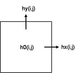
  • h0 (imin:imax,jmin:jmax)
  • hx (imin:imax,jmin:jmax)
  • hy (imin:imax,jmin:jmax)

• State variables

  • ssh (imin:imax,jmin:jmax) : sea surface height
  • u (imin:imax,jmin:jmax) : barotropic zonal velocity (from row calculation at t+dt/2)
  • uz (kmax,imin:imax,jmin:jmax) : 3D zonal velocity (from row calculation at t+dt/2)
  • v : barotropic zonal velocity (from column calculation at t+dt/2)
  • vz (kmax,imin:imax,jmin:jmax) : 3D meridional velocity (from column calculation at t+dt/2)
  • sal (kmax,imin:imax,jmin:jmax) : salinity
  • temp (kmax,imin:imax,jmin:jmax) : temperature
  • cv_wat (nb_var,kmax,imin:imax,jmin:jmax) : substance

Turbulence models : nz,kz for Vertical Mixing

\(\frac{1}{D}\frac{\partial(\frac{nz}{D}\frac{\partial u}{\partial \sigma })}{\partial \sigma }\)

• 0 equations : turb_nbeq=0

  • cst : nz , kz constant ! turb_0eq_option = 1

  • Prandt model

    : viscosite=f(u*) constant mixing length ! turb_0eq_option = 2

    • \(nz=u^*\frac{H}{15}*\sigma\sqrt{1-\sigma}\)
    • \(u^*=\frac{0.4}{\log{\frac{(\sigma+1) H}{z_0}}} u_{bottom}\)

  • Quetin model

    : based on density stratification : no constant mixing length ! turb_0eq_option = 3

    • \(nz=l^2\frac{\partial u}{\partial z}\)
    • \(kz=f(Ri)l^2\frac{\partial u}{\partial z}\)
    • l analytical

  • Pacanovski et Philander, 1981

    : ! turb_0eq_option = 4

    • \(nz=\frac{\nu_0}{(1+\alpha Ri)^n}+\nu_b\)
    • \(kz=\frac{\nu}{(1+\alpha Ri)}+k_b\)
    • \(Ri=\frac{\frac{\partial b}{\partial z}}{|\frac{\partial U}{\partial z}|^2}\)

• 1 equation : turb_nbeq=1

  • Gaspard et al, 1990 :

    • \(nz,kz=f(ect,l)\)
    • ect computed and l evaluated

• 2 equations : turb_nbeq=2

  • Warner et al. 2005

    • \(nz,kz=f(k,kl,l)\)
    • k,kl computed and l evaluated

  • 4 turbulence closure models

    • k-kl

      : turb_2eq_option = 1

      • Close to Mellor–Yamada level 2.5 scheme of Mellor et Yamada (1974, 1982)

    • k–ε

      : turb_2eq_option = 2

      • Jones and Launder (1972), Launder and Sharma (1974)
      • Burchard et al. (1998), Burchard and Bolding (2001)

    • k-ω

      : turb_2eq_option = 3

      • Kolmogorov (1942), Saffman (1970), Saffman and Wilcox (1974), Umlauf et al. (2003)

    • GLS

      : generic length scale ! turb_2eq_option = 4

      • Umlauf and Burchard (2003)

Parametrization of the bathymetry

• hminim marks off the coastline beacuse it is the minimum value of the bathymetri (hx,hy)
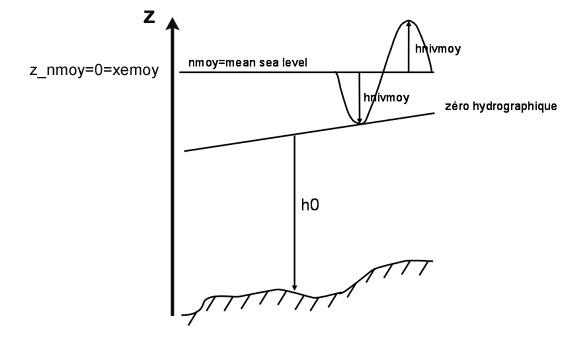
• hminim= -max (‘|’hnivmoy’|’) along the coastline
• In microtidal area, if the reference for the bathymetry is the level of lowest astronomical tides, the shift hnivmoy is applied to the inital bathymetric value. Then, the tidal signal evolves around the mean sea level. All along the coast, hminim is equal to hnivmoy and marks the coast line.
• The parameter xemoy may be used when the model vertical reference of the bathymetry derives from a preexisting level network (IGN 69, NGF..), that differs from the hydrographic zero (level of lowest astronomical tides)

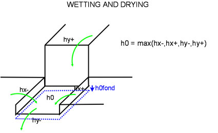
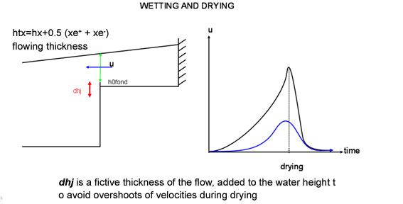
Note on wetting and drying

• h0fond is a residual thickness used to ensure h0+xe keeps positive.
• As the continuity scheme is not positive definite, it might be possible to export more water mass than available in the cell during the drying

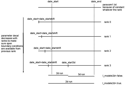
Parametrization of the run period